Timing of River Ice Formation and Break-Up in New Brunswick
Half a dozen years ago, I did a summer work term for Hydro-Com Technologies. I had a good experience there and learned a lot. One project I was involved in while I was there was an analysis in trends in rivers in New Brunswick related to streamflow, ice break-up, etc. A portion of this work ended up getting presented at a conference. This seemed like a good time to look back at this project, being in the middle of another flood season.
The paper was presented at the 15th Workshop of the Committee of River Ice Processes and the Environment and can be found here. Here is the abstract:
Analyses were performed on hydrometric data for 13 selected hydrometric sites in New Brunswick to detect trends in ice season characteristics (earliest and latest dates of ice effects on hydrometric records, the number of days with ice effect, freeze-up and breakup flows and the estimated number of break-up events each year). The coefficient of determination, r^2, and the p-value for the slope of a linear regression line were used to assess the significance of any possible trends in the data. The coefficient of determination, r^2, is a measure of the degree of relationship between two variables. The slope of the regression line depicts the average rate of change in a variable over time, and its probability indicates if the slope value is statistically significantly different from zero. In the absence of more specific information, the notation of a backwater effect in the hydrometric records was used to evaluate the beginning and end of periods of ice, the number of ice-covered periods and the duration of the ice season. The existence of a backwater effect is indicated in Environment Canada’s HYDAT database by the symbol “B”. It was found that trends in hydrologic data are beginning to appear in the hydrometric records. As the climate continues to change, trends in hydrologic data are expected to be more evident and statistically significant.
(Burrell, Arisz, Scott, and DeVenney, 2009).
One of the things that the results of this study suggested was a trend towards ice break-ups occurring earlier in the year (see Figure 5).
If you're just interested in my latest results, skip down to the Results & Interpretation section; the intervening portion will be pretty heavy on statistical methods.
Looking back, I'd change some things about the statistical approach (although I do really like how we presented the results graphically overlaid on a map of the province) based on things I've learned in the intervening years:
- Not using Excel—one thing I remember quite vividly about this project was the enormous amount of time I spent getting the data into the forms we wanted. The datasets came with just the daily flows and a symbol that indicated whether a backwater effect existed; I had to work it into seasonal flows and dates of ice formation and break-up, etc. Using a computer that was old even at the time (2008), some of the spreadsheet functions I used would sputter away for minutes on the tens of thousands of rows of data.
- Using more appropriate statistics—hydrological data often doesn't follow a normal distribution and the responses between different variables could be non-linear. For these reasons, non-parametric statistics may be better than the ones we used in the study above.
- Using more appropriate confidence levels—i.e. 90% or 95%.
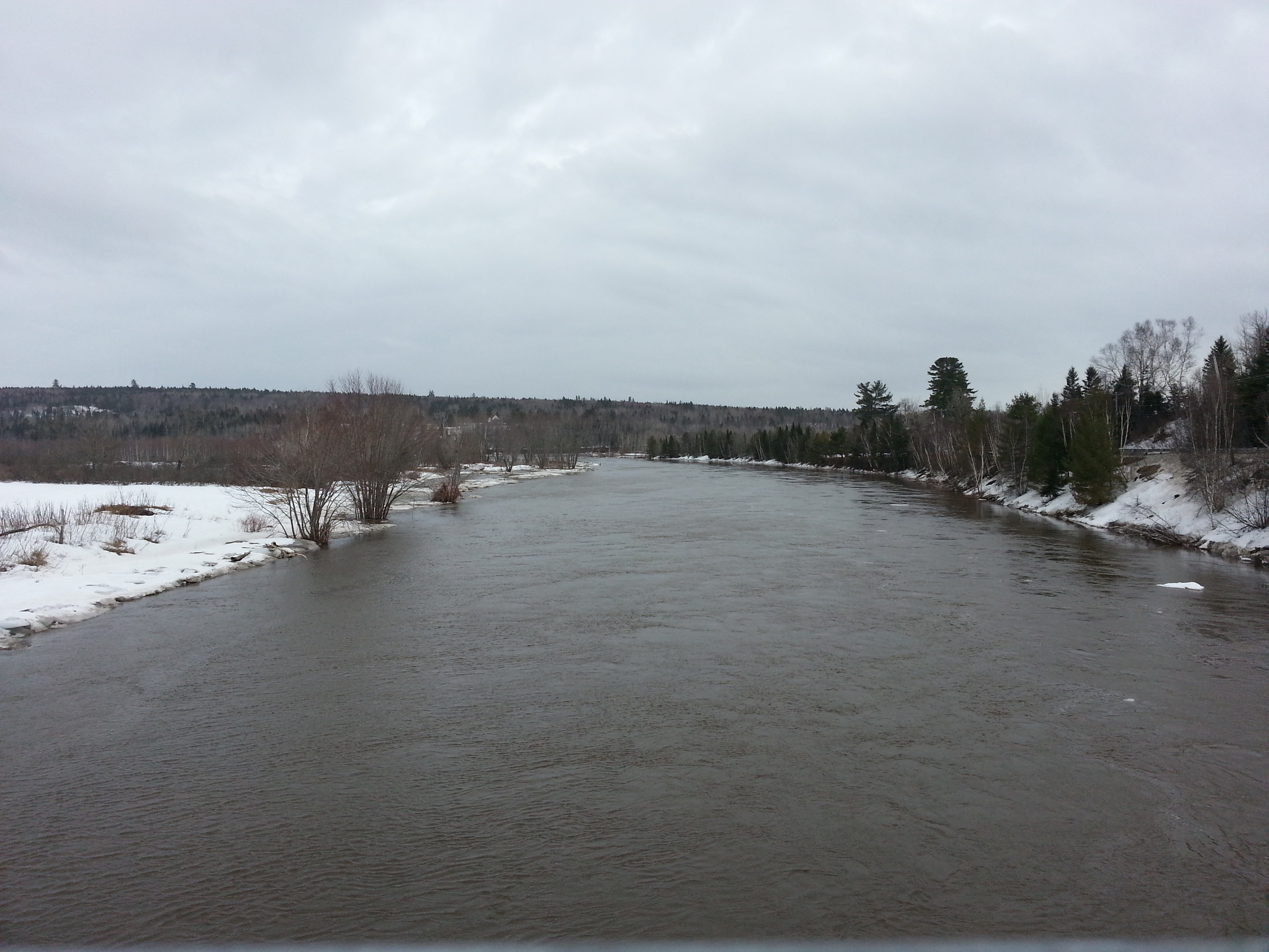
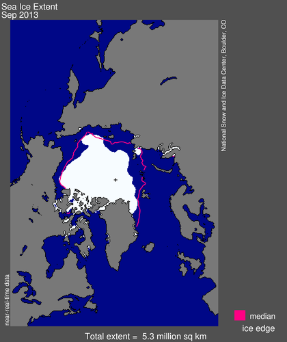
For this post, I retrieved data for one of the hydrological stations used in the study above and did some new calculations in R (using the RStudio console). Archived hydrometric data for Canada is freely available from the Water Survey of Canada. The station I chose to look at is 01AL002 – Nashwaak River at Durham Bridge, due to its proximity to my city. Archived streamflow data is available up to 2010 for this station; its current water level can be checked here though. While I was at it, I also downloaded a couple of common climate change datasets for comparison: the global temperature anomaly from James Hansen's group and the Arctic sea ice extent (September) from the National Snow and Ice Data Center. The temperature anomaly was in units of 0.01 degrees Celsius (i.e. +21 instead of +0.21 deg C), which I found a bit misleading, so I changed it in my calculations. See the bottom of this post for pictures of the Nashwaak River from Durham Bridge and the Arctic Sea Ice Extent in September 2013.
After obtaining the variables I was interested in from the data set (the hardest part), I applied some non-parametric statistics to conduct the analysis. Instead of the traditional correlation coefficient, I used the Spearman correlation coefficient, to look for relationships between variables. For example, a positive correlation between a variable and the year suggests that it is increasing, but says nothing about the magnitude or whether it is a linear trend. I also used the Mann-Whitney U Test to check whether the second half of each data set was significantly different than the first half, indicating an increase or decrease.
I did these calculations in an interactive session, but the commands could easily be put into a script and quickly applied to data from other stations—a major advantage over doing analyses like this in a spreadsheet.
Below, I've included some sections of my session in R (condensed in places) followed by some of the results and a few photos.
Importing data and doing some initial checks
This part is pretty self-explanatory.
> NashwaakR <- read.csv("01AL002_DailyQ.csv",header=TRUE)
> SeaIce <- read.csv("ArcticSeaIceSept.csv",header=TRUE)
> TempAnom <- read.csv("GISS_LOTI_TempAnom.csv",header=TRUE)
> summary(NashwaakR)
       ID            Value         SYM
 01AL002:17897   Min.   :   2.16    :11517
                 1st Qu.:   9.54   A:  109
                 Median :  18.40   B: 5943
                 Mean   :  35.83   E:  328
                 3rd Qu.:  40.20
                 Max.   :1150.00
> summary(SeaIce)
...
> summary(TempAnom)
...
> by(NashwaakR$Value,NashwaakR$Year,max)
NashwaakR$Year: 1962
[1] 148
---------------------------------------------------------------------------------------
NashwaakR$Year: 1963
[1] 467
---------------------------------------------------------------------------------------
NashwaakR$Year: 1964
[1] 408
...
Generating some variables of interest
The variable names I used here are:
- Year = a year between 1979 – 2010 (the period covered by all the datasets
- SpringRunoff = the maximum flow recorded in each year (assumed to be the spring flooding, although the peak flow occurred in the fall in a few years)
- Note that all of the river-related variables are for the Nashwaak River at Durham Bridge
- FloodDate = the day in the year (a number from 1 – 366) on which the peak flow occurred
- IceDays = the total number of days in each winter (i.e. the winter/spring in one year and the fall in the year before) with a backwater effect
- LastIce = the latest day in the year (but not in the fall) in which a backwater effect was recorded
- ArcticIceExtent = the area encompassed by sea ice in the Arctic Ocean in September (not necessarily at 100% coverage)
- GlobalTempAnom = the difference between the average global temperature for each year and the average temperature in the baseline period, in degrees Celsius.
(It took some trial and error to get the statements in the "for" loops right).
> Year <- seq(1979,2010,1)
> summary(Year)
   Min. 1st Qu.  Median    Mean 3rd Qu.    Max.
   1979    1987    1994    1994    2002    2010
> Index <- seq(1,length(Year),1)
> max(Index)
[1] 32
> max(NashwaakR$Value[NashwaakR$Year==1967])
[1] 247
> SpringRunoff <- numeric(length(Index))
> for (i in Index)
+ SpringRunoff[i] <- max(NashwaakR$Value[NashwaakR$Year==Year[i]])
> summary(SpringRunoff)
   Min. 1st Qu.  Median    Mean 3rd Qu.    Max.
  149.0   277.2   341.0   394.1   471.5  1150.0
...
> FloodDate <- numeric(length(Index))
> Index2 <- seq(1,length(NashwaakR$JulianDay),1)
> IsAnnualMax <- numeric(length(Index2))
> for (i in Index2)
+ IsAnnualMax[i] <- NashwaakR$Value[i] == max(NashwaakR$Value[NashwaakR$Year==NashwaakR$Year[i]])
> summary(IsAnnualMax)
   Mode   FALSE    TRUE    NA's
logical   17847      50       0
> summary(NashwaakR$JulianDay[IsAnnualMax==TRUE])
   Min. 1st Qu.  Median    Mean 3rd Qu.    Max.
   15.0   106.0   113.5   149.0   126.5   362.0
> FloodDate <- NashwaakR$JulianDay[IsAnnualMax==TRUE & NashwaakR$Year>=Year[1]]
> summary(FloodDate)
   Min. 1st Qu.  Median    Mean 3rd Qu.    Max.
   15.0   100.0   112.5   148.8   121.2   348.0
> IceDays <- numeric(length(Index))
> for (i in Index)
+ IceDays[i] <- sum(NashwaakR$SYM=="B" & NashwaakR$Year==Year[i] & NashwaakR$JulianDay<185) + sum(NashwaakR$SYM=="B" & NashwaakR$Year==(Year[i]-1) & NashwaakR$JulianDay>=185)
> summary(IceDays)
   Min. 1st Qu.  Median    Mean 3rd Qu.    Max.
   90.0   107.8   116.5   117.7   131.2   141.0
> LastIce <- numeric(length(Index))
> for (i in Index)
+ LastIce[i] <- max(NashwaakR$JulianDay[NashwaakR$Year==Year[i] & NashwaakR$SYM=="B" & NashwaakR$JulianDay<185])
> summary(LastIce)
   Min. 1st Qu.  Median    Mean 3rd Qu.    Max.
  68.00   85.00   96.00   92.12   99.00  112.00
...
> ArcticIceExtent <- SeaIce$extent[SeaIce$year<=2010]*1000000
> length(ArcticIceExtent)
[1] 32
> summary(ArcticIceExtent)
   Min. 1st Qu.  Median    Mean 3rd Qu.    Max.
4300000 6110000 6650000 6580000 7300000 7880000
> GlobalTempAnom <- TempAnom$Glob[TempAnom$Year>=1979 & TempAnom$Year<=2010]/100
> length(GlobalTempAnom)
[1] 32
> summary(GlobalTempAnom)
   Min. 1st Qu.  Median    Mean 3rd Qu.    Max.
 0.0800  0.2375  0.3850  0.3803  0.5450  0.6600
Doing some calculations
(For clarity, I've deleted warning messages, which are mainly about having to use an approximation in the presence of ties). These results are summarized and interpreted in the next section.
> cor(LastIce,FloodDate,method="spearman")
[1] 0.3950200
> cor(LastIce,IceDays,method="spearman")
[1] 0.6604506
> cor(SpringRunoff,IceDays,method="spearman")
[1] 0.0680422
> cor(SpringRunoff,LastIce,method="spearman")
[1] -0.06922524
> cor(SpringRunoff,FloodDate,method="spearman")
[1] 0.1916904
> cor.test(Year,SpringRunoff,method="spearman")

	Spearman's rank correlation rho

data:  Year and SpringRunoff
S = 3748, p-value = 0.08142
alternative hypothesis: true rho is not equal to 0
sample estimates:
      rho
0.3130499

> cor.test(SpringRunoff,FloodDate,method="spearman")

	Spearman's rank correlation rho

data:  SpringRunoff and FloodDate
S = 4410.137, p-value = 0.2933
alternative hypothesis: true rho is not equal to 0
sample estimates:
      rho
0.1916904

> cor.test(Year,FloodDate,method="spearman")

	Spearman's rank correlation rho

data:  Year and FloodDate
S = 4169.939, p-value = 0.1940
alternative hypothesis: true rho is not equal to 0
sample estimates:
     rho
0.235715

> cor(ArcticIceExtent,GlobalTempAnom,method="spearman")
[1] -0.767009
> cor.test(ArcticIceExtent,GlobalTempAnom,method="spearman")

	Spearman's rank correlation rho

data:  ArcticIceExtent and GlobalTempAnom
S = 9640.801, p-value = 3.052e-07
alternative hypothesis: true rho is not equal to 0
sample estimates:
      rho
-0.767009


> cor(Year,ArcticIceExtent,method="spearman")
[1] -0.8188067
> cor(Year,GlobalTempAnom,method="spearman")
[1] 0.8750345
> cor(GlobalTempAnom,SpringRunoff,method="spearman")
[1] 0.3111763
> cor(GlobalTempAnom,FloodDate,method="spearman")
[1] 0.1539732
> cor.test(GlobalTempAnom,SpringRunoff,method="spearman")

	Spearman's rank correlation rho

data:  GlobalTempAnom and SpringRunoff
S = 3758.222, p-value = 0.083
alternative hypothesis: true rho is not equal to 0
sample estimates:
      rho
0.3111763


> cor(ArcticIceExtent,IceDays,method="spearman")
[1] 0.06859869
> cor(ArcticIceExtent,LastIce,method="spearman")
[1] -0.0519696
> median(Year)
[1] 1994.5
> wilcox.test(GlobalTempAnom[Year<=1994],GlobalTempAnom[Year>1994])

	Wilcoxon rank sum test with continuity correction

data:  GlobalTempAnom[Year <= 1994] and GlobalTempAnom[Year > 1994]
W = 3, p-value = 2.674e-06
alternative hypothesis: true location shift is not equal to 0


> wilcox.test(ArcticIceExtent[Year<=1994],ArcticIceExtent[Year>1994])

	Wilcoxon rank sum test with continuity correction

data:  ArcticIceExtent[Year <= 1994] and ArcticIceExtent[Year > 1994]
W = 229.5, p-value = 0.0001407
alternative hypothesis: true location shift is not equal to 0


> wilcox.test(LastIce[Year<=1994],LastIce[Year>1994])

	Wilcoxon rank sum test with continuity correction

data:  LastIce[Year <= 1994] and LastIce[Year > 1994]
W = 129.5, p-value = 0.9699
alternative hypothesis: true location shift is not equal to 0


> wilcox.test(IceDays[Year<=1994],IceDays[Year>1994])

	Wilcoxon rank sum test with continuity correction

data:  IceDays[Year <= 1994] and IceDays[Year > 1994]
W = 138.5, p-value = 0.7061
alternative hypothesis: true location shift is not equal to 0


> wilcox.test(SpringRunoff[Year<=1994],SpringRunoff[Year>1994])

	Wilcoxon rank sum test

data:  SpringRunoff[Year <= 1994] and SpringRunoff[Year > 1994]
W = 101, p-value = 0.3226
alternative hypothesis: true location shift is not equal to 0

> wilcox.test(FloodDate[Year<=1994],FloodDate[Year>1994])

	Wilcoxon rank sum test with continuity correction

data:  FloodDate[Year <= 1994] and FloodDate[Year > 1994]
W = 113.5, p-value = 0.5974
alternative hypothesis: true location shift is not equal to 0


> wilcox.test(Year[Year<=1994],Year[Year>1994])

	Wilcoxon rank sum test

data:  Year[Year <= 1994] and Year[Year > 1994]
W = 0, p-value = 3.327e-09
alternative hypothesis: true location shift is not equal to 0
> length(Year)
[1] 32
To double-check the results from R, I looked up the 90% significance level for the Spearman correlation with 32 data points in a table: 0.306.
Results & Interpretation
The following Spearman correlations were statistically significant at a 90% level:
- The date of the last ice effect with the date of the flood crest—as one would expect, since ice break-up and spring flooding happen around the same time as each other each year
- The date of the last ice effect with the number of days of ice effect each winter—a longer winter means river ice lasts later and is around longer
- The peak flow during a year (usually in the spring) with the year—this was a positive correlation, suggesting increasing magnitudes of the peak flow (although it says nothing about the magnitude of the trend)
- Arctic sea ice extent in September with the global annual temperature anomaly—this was a negative correlation, meaning that a higher temperature corresponds with more ice melting in the Arctic ocean during the summer
- Arctic sea ice extent in September and the global annual temperature anomaly both had significant correlations with the year
- The peak flow during a year with the global annual temperature anomaly
By the Mann-Whitney U-test, only the global temperature anomaly and the Arctic sea ice extent in September had statistically significant differences before vs. after 1994 (the midpoint of the dataset). Notably, the peak flow during a year and the date of the last ice effect at the hydrometric station did not show significant differences between the early and recent years of the dataset according to this test. Trends in environmental data can take a long time to become fully apparent.
As we're seeing this year, the most impacting floods are often due to ice jams, which are even more random than the date of ice break-up or the peak flow volumes. As you read this post, please keep in mind as well, that rivers are impacted by a lot more than climate trends (e.g. land use changes). In my opinion, the way to deal with the uncertainty around flood risks, etc. is to make sure we have robust infrastructure, good preparedness, and design resiliency into the built environment.
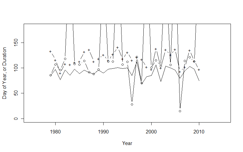
(The line in the graph is the day of the last ice effect, the plus sign is the number of ice days, and the circle is the flood crest date (sometimes in the fall, off the graph as shown)).