7 Excel Functions and Features to Know
In this post, I thought I'd share some tools and features in Microsoft Excel that I've come across over the years. This post is not intended as a comprehensive tutorial on any of these features; rather, it can be a starting point for learning more about the ones that sound useful to you.
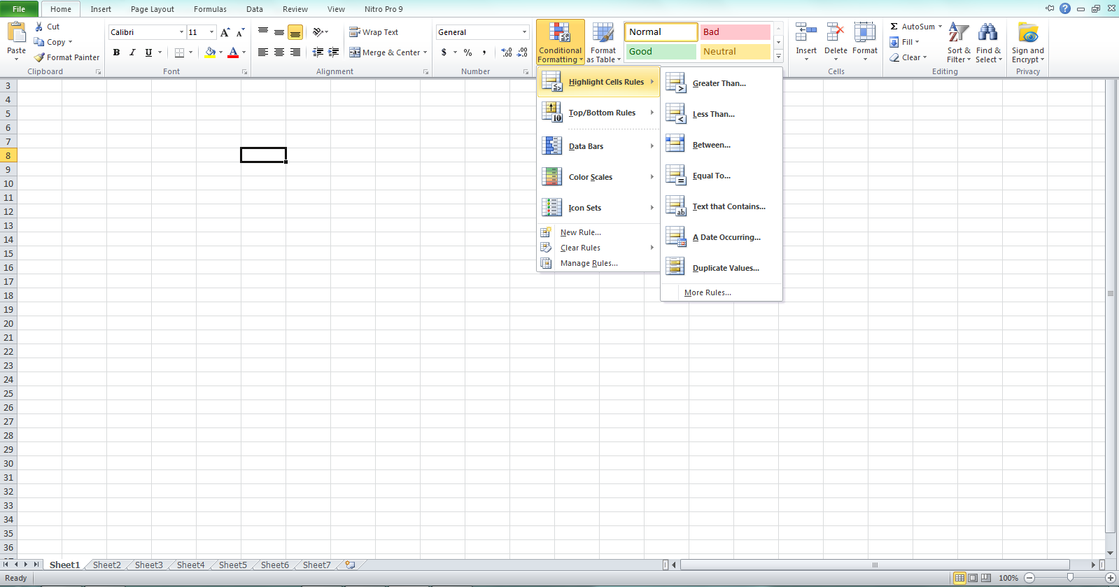
1. Conditional formatting
I'm sure most Excel users are already aware of this tool, but I'm including it in this list because of how frequently useful it is. It allows you to highlight cells (or apply other formatting such as bold-face or coloured fonts) based on their values. It can make it much faster to identify values in a list that are over a threshold value, for example.
Find it under: Home – Conditional Formatting
2. Conditional counting/summation/averaging
This set of functions allows very basic statistics (the count, sum total, or average) for a set of numbers to be calculated for only the elements that meet a certain condition (or add an "S" to the end of the function name to apply multiple conditions). For example, you can take the average of only numbers ">0" (include the quote marks in the condition). The condition(s) can even apply to a different column than the data being counted/summed/averaged.
=COUNTIF(), =SUMIF(), =AVERAGEIF()
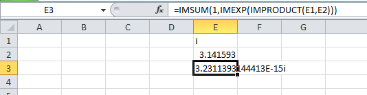
3. Complex numbers
Complex numbers (of the form 1+2i) can be used in Excel. However, they don't integrate well with the other spreadsheet functions—at least in the current version of Excel:
=SQRT(-1)generates an error rather than an imaginary number- Specialized functions (all beginning with
=IM...) must be used even for functions as basic as addition - Number formatting and rounding cannot be applied (as far as I've found) so numbers will be displayed with up to 15 significant digits and floating point errors can creep in quite easily
Here is an example showing Euler's identity calculated in Excel. The result should be zero, but the imaginary coefficient was left with a floating-point inaccuracy of around 3 × 10-15.
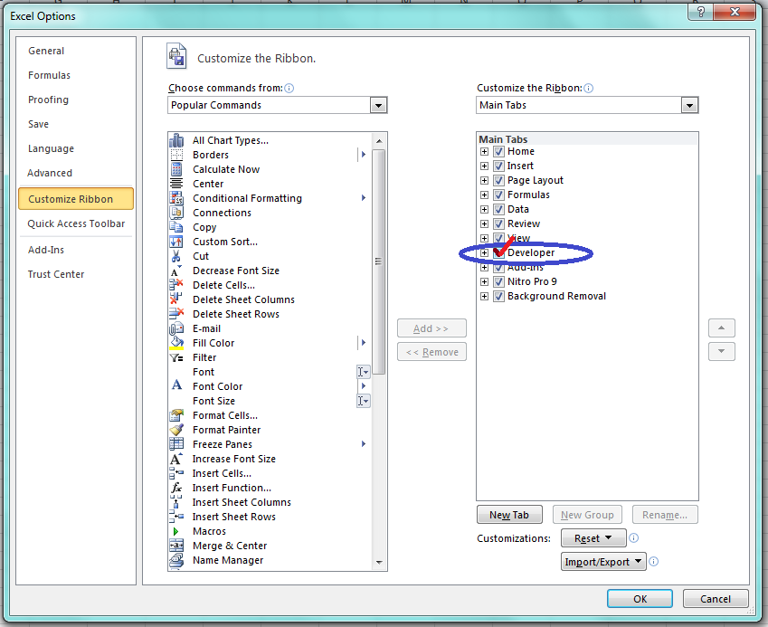
4. Slider bars
To use this feature, you have to first activate the Developer menu:
File – Options – Customize Ribbon
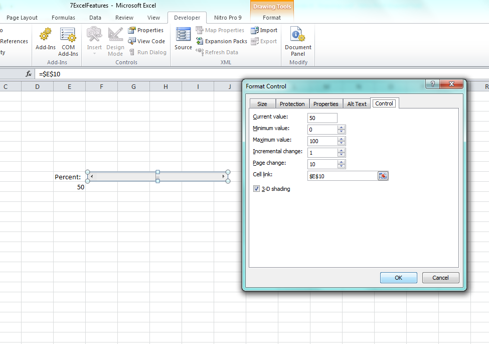
From the Developer toolbar, you can insert different control buttons to make a spreadsheet interactive for end users.
To draw a slider bar, select: Developer – Insert – Scroll Bar (Form control)
Once the bar is drawn, right click on it to format its control functions. You can set the range, the increment value, and pick a cell in which to display/link the output. In the example shown, a slider bar has been drawn and configured to input a percent value, limited to a range of 0 – 100 and whole numbers within that range. Users can then use the slider bar to adjust the value within the set limits. This tool is thus a way to control the inputs to spreadsheet functions to acceptable/meaningful values.
See also: Data – Data Validation – Data Validation for other ways to restrict cell values to certain formats (Whole Numbers) or values from a list/drop-down menu.
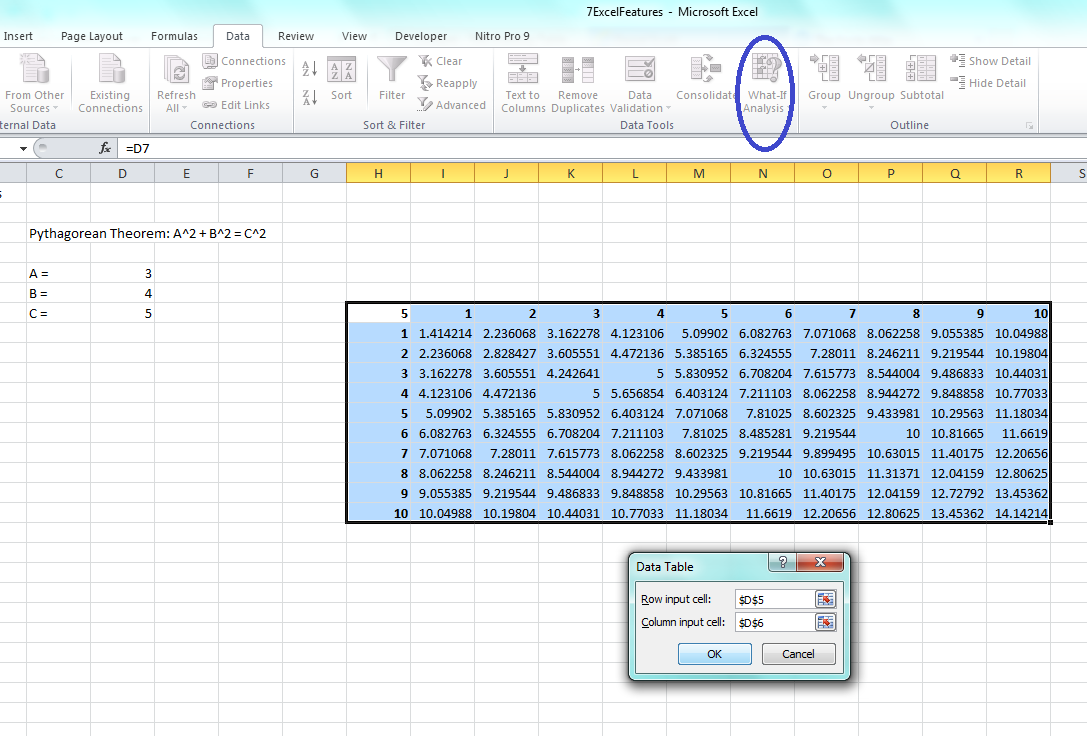
5. What-if analysis
If you have a spreadsheet set up to do some calculations on some input cells and want to quickly see how a result would change if a couple of the input values were changed (e.g. for a sensitivity analysis, or running different scenarios), this feature allows you to automatically generate a data table that will do just that.
This tool is found under: Data – What-If Analysis – Data Table, but you need to prepare the table in a standardized format first:
- In the top left cell of where the table will go, link to the result cell from where the calculation is already set up (in the example shown, H7 is linked to D7)
- Along the top row enter values (numbers, not formulas) to be used for one of the inputs
- Along the left column enter values (numbers, not formulas) to be used for the other input
- Select the whole table (the interior space is still blank at this point), then click on the data table button; identify which cells contain the inputs that the top row and left column values are to be substituted for in the pop-up dialogue
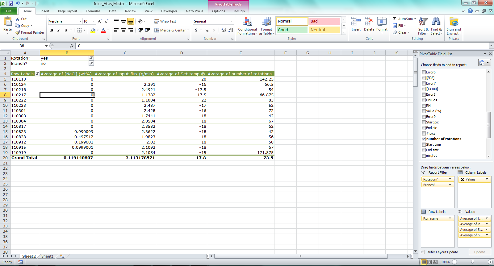
6. Pivot tables
Entire books could be—and have been—written about pivot tables in Excel, so this is the barest of introductions to the topic. Basically, pivot tables allow you to explore and summarize data in an interactive manner.
To generate a pivot table, select the source data you want and click: Insert – Pivot Table. Initially the pivot table will be empty. You can drag-and-drop (in a pane on the right hand side of the window) the various parameters (taken from column titles in the source data) to be filters, row labels, column labels, or values in the pivot table. Any parameter that you want displayed in the table should be dragged to the "Value" box; the row and column boxes dictate how the table is structured, and the filter box lets you narrow down which entries will be included in the pivot table based on the value of categorical parameters.
When a parameter is placed in the "Values" box, it starts off being summarized by its count. If you instead want to see the sum or average of all the entries that fit under each row/column label, click the arrow beside a parameter of interest and edit the "Value field settings" to apply a sum or average (or other) function. Number formats can also be applied here.
The example shown here uses data from the Icicle Atlas.
7. Array functions
Finally, Array Functions can be a big time and space saver if you know how to use them. Unlike regular functions, they require the user to press ctrl + shift + enter instead of just enter after typing them.
An example of an array function is =MMULT() for matrix multiplication (also look for other matrix functions that start with =M...). They can also be used for applying calculations across a range of cells that normally take a single cell as input.
For my next post, I plan to do something fun with complex numbers in Excel.