ASM1 in Octave
This post contains an implementation of the IWA's Activated Sludge Model No. 1 (ASM1) in octave.
Models are a widely-used tool in the design and operation of wastewater treatment systems. For my job, I use a commercial simulator, but I thought it would be a useful exercise to write an implementation of a simpler model (i.e. ASM1) on my own—to better understand how these models work "under-the-hood". Most wastewater models have a similar structure, built around the "Gujer matrix", which relates the rates of various processes to the changes they cause on different components.
Because the model was already defined and expressed in matrix form, I decided to code a script for it in octave. Octave is an open-source computer language that is highly similar to Matlab; vectors and matrices are its default data type, so it is well-suited for this application.
My script is included below. It is written for batch kinetics, so the mass balance only includes transformations of the initial components, not any flow in or out of the reactor. The dissolved oxygen concentration is fixed (as in a respirometer or a system with DO control) at 2.0 mg/L. The value could be changed to zero to simulate denitrification.
Following the code, I've included an example of its use with input values and a few output graphs.
Reminder: This blog is solely my own and may not reflect the views of my employer or association(s). If you use this code, you do so at your own risk.
The Code
% ASM1 (IWA's "Activated Sludge Model No. 1") has a stoichiometric matrix, S (8x13),
% a vector of process rates, Rho (8x1), and a vector of component conversion
% rates, r (1x13).
% S will be fixed in each run of the model while Rho and r depend on the current
% concentrations and will thus change at each time-step (dt).
%
%%% Calculation Procedure
% 1. Read in the initial concentrations, Ci (1x13 vector)
% 2. Set the values of the various coefficients (i_, f_, Y_, k_, etc.)
% 3. Initialize the stoichiometric matrix, S
% 4. For an appropriate time-step, dt, do the following calculations
% * Use Ccurr to determine Rho
% * r = Rho' x S; (verify with rules of matrix multiplication???)
% * Ccurr = Ccurr + r x dt;
% * For Oxygen, Ccurr(8), it may be better to modify to have continuous input and record the uptake rate
% * At a suitable interval (Interval), record Ccurr in Ct (N x 13)
% 5. When the simulation is finished, Ct can be used for output. A plot should be produced.
%
%% NOTE: This script is only set up for batch kinetics in a single reactor.
%
% Table numbers refer to IWA Scientific and Technical Report No. 9.
%
%% Read-in initial concentrations
Ci = zeros(1,13);
fprintf("Enter intial concentrations of each model component, in mg/L.\n");
Ci(1,1) = input("Soluble inert organic matter, Si: \n");
Ci(1,2) = input("Readily biodegradable substrate, Ss: \n");
Ci(1,3) = input("Particulate inert organic matter, Xi: \n");
Ci(1,4) = input("Slowly biodegradable substrate, Xs: \n");
Ci(1,5) = input("Active heterotrophic biomass, Xb,h: \n");
Ci(1,6) = input("Active autotrophic biomass, Xb,a: \n");
Ci(1,7) = input("Particulate decay products, Xp: \n");
Ci(1,8) = 2.0; % Assume a fixed O2 concentration and calculate the OUR.
Ci(1,9) = input("Nitrate- and nitrite- nitrogen, Sno: \n");
Ci(1,10) = input("Ammonia-nitrogen, Snh: \n");
Ci(1,11) = input("Soluble biodegradable organic nitrogen, Snd: \n");
Ci(1,12) = input("Particulate biodegradable organic nitrogen, Xnd: \n");
Ci(1,13) = input("Alkalinity - molar units, Salk: \n");
Ccurr = Ci;
%% Set the values of the coefficients and constants
% Default values from Table 5, p. 24
YA = 0.24; % g cell COD formed/ g N oxidized
YH = 0.67; % g cell COD formed/ g COD oxidized
fp = 0.08; % dimensionless, fraction of biomass going to inert products
iXB = 0.086; % g N in biomass / g COD in biomass
iXE = 0.06; % g N in endogenous mass/ g COD in endogenous mass
MuH = 6.0; % per day; heterotroph growth
Ks = 20.0; % g COD/m^3; COD half-saturation coefficient
KOH = 0.20; % g O2/m^3; oxygen switch
KNO = 0.50; % g NO3-N/m^3; nitrate switch
bH = 0.62; % per day; heterotroph decay
bA = 0.10; % per day; autotroph decay
Etag = 0.8; % anoxic growth discount
Etah = 0.4; % anoxic hydrolysis discount
kh = 3.0; % g slowly biodegradable COD/g cell COD/day; hydrolysis rate
KX = 0.03; % g slowly biodegradable COD/g cell COD; hydrolysis half-saturation coeff.
MuA = 0.80; % per day; autotroph growth
KNH = 1.0; % g NH3-N/m^3; ammonia half-saturation coefficient
KOA = 0.4; % g O2/m^3; oxygen switch
ka = 0.08; % m^3/g COD/d; ammonification rate
%% Initialize the stoichiometric matrix
S = zeros(8,13);
%process 1: aerobic growth of heterotrophs
S(1,2) = -1/YH;
S(1,5) = 1;
S(1,8) = -(1-YH)/YH;
S(1,10) = -iXB;
S(1,13) = -iXB/14;
%process 2: anoxic growth of heterotrophs
S(2,2) = -1/YH;
S(2,5) = 1;
S(2,9) = -(1-YH)/(2.86*YH);
S(2,10) = -iXB;
S(2,13) = ((1-YH)/(14*2.86*YH)) - iXB/14;
%process 3: aerobic growth of autotrophs
S(3,6) = 1;
S(3,8) = -(4.57-YA)/YA;
S(3,9) = 1/YA;
S(3,10) = -iXB - (1/YA);
S(3,13) = -(iXB/14) - (1/(7*YA));
%process 4: decay of heterotrophs
S(4,4) = 1-fp;
S(4,5) = -1;
S(4,7) = fp;
S(4,12) = iXB - fp*iXE;
%process 5: decay of autotrophs
S(5,4) = 1-fp;
S(5,6) = -1;
S(5,7) = fp;
S(5,12) = iXB - fp*iXE;
%process 6: ammonification
S(6,10) = 1;
S(6,11) = -1;
S(6,13) = 1/14;
%process 7: hydrolysis of entrapped organics
S(7,2) = 1;
S(7,4) = -1;
%process 8: hydrolysis of entrapped nitrogen
S(8,11) = 1;
S(8,12) = -1;
%% Simulate with suitable time-step;
dt = 1/1440; %in days
Interval = 1/24; %in days
maxtime = input("How long should the simulation run (in days)? \n");
Record = 1; %index of Ct
Rho = zeros(8,1); %Create Rho and r as empty vectors
r = zeros(1,13);
for time = 0:dt:maxtime
%Record Ct
if mod(time,Interval)==0
Ct(Record,:) = Ccurr; %Save the concentrations in a matrix for output
Ct(Record,8) = r(1,8); %Replace the O2 concentration (constant) with the OUR in mg/L*d.
Timet(Record,1) = time; %Save the times in a vector for output
Record = Record + 1; %increment the index
end
%Calculate Rho
Rho(1,1) = MuH*(Ccurr(1,2)/(Ks+Ccurr(1,2)))*(Ccurr(1,8)/(KOH+Ccurr(1,8)))*Ccurr(1,5);
Rho(2,1) = MuH*(Ccurr(1,2)/(Ks+Ccurr(1,2)))*(KOH/(KOH+Ccurr(1,8)))*(Ccurr(1,9)/(KNO+Ccurr(1,9)))*Etag*Ccurr(1,5);
Rho(3,1) = MuA*(Ccurr(1,10)/(KNH+Ccurr(1,10)))*(Ccurr(1,8)/(KOH+Ccurr(1,8)))*Ccurr(1,6);
Rho(4,1) = bH*Ccurr(1,5);
Rho(5,1) = bA*Ccurr(1,6);
Rho(6,1) = ka*Ccurr(1,11)*Ccurr(1,5);
Rho(7,1) = kh*((Ccurr(1,4)/Ccurr(1,5))/(KX+(Ccurr(1,4)/Ccurr(1,5))))*((Ccurr(1,8)/(KOH+Ccurr(1,8)))+Etah*(KOH/(KOH+Ccurr(1,8)))*(Ccurr(1,9)/(KNO+Ccurr(1,9))))*Ccurr(1,5);
Rho(8,1) = Rho(7,1)*Ccurr(1,12)/Ccurr(1,4);
%Calculate r and Ccurr
r = Rho' * S;
Ccurr = Ccurr + r*dt;
Ccurr(1,8) = Ci(1,8); % reset O2 concentration
end
%% Plot the results
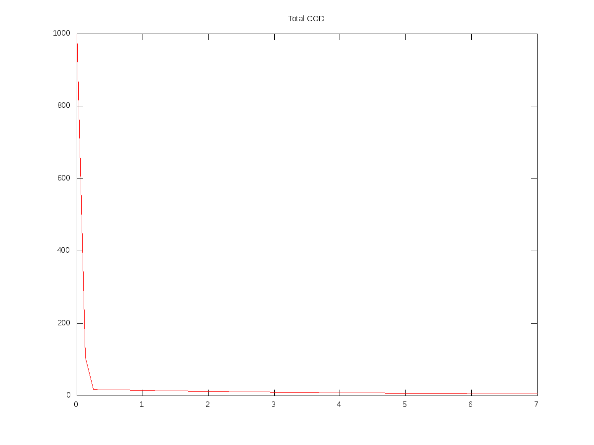
tCOD = Ct(:,1) + Ct(:,2) + Ct(:,3) + Ct(:,4);
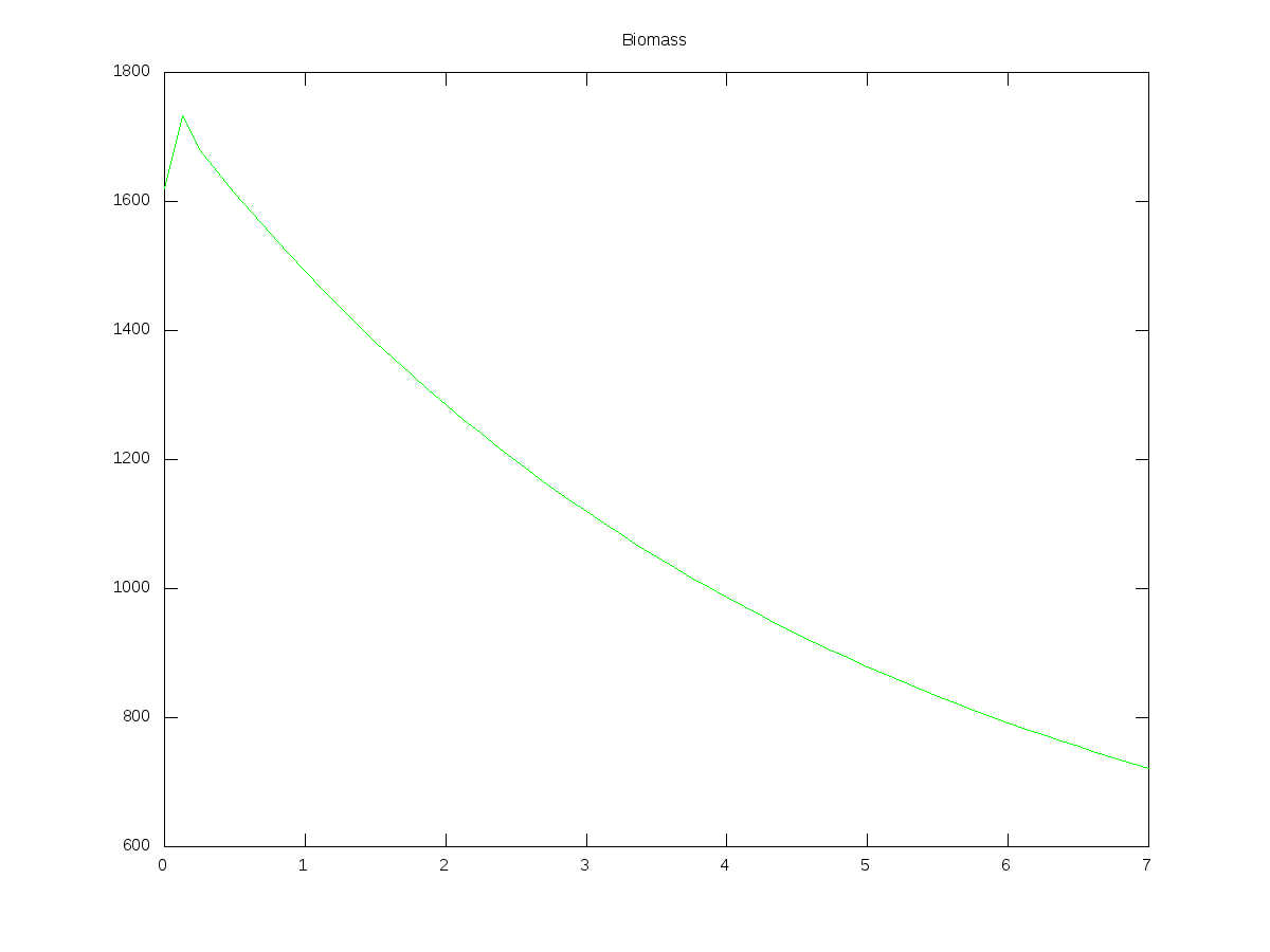
MLVSS = (Ct(:,3) + Ct(:,4) + Ct(:,5) + Ct(:,6) + Ct(:,7))/1.42;
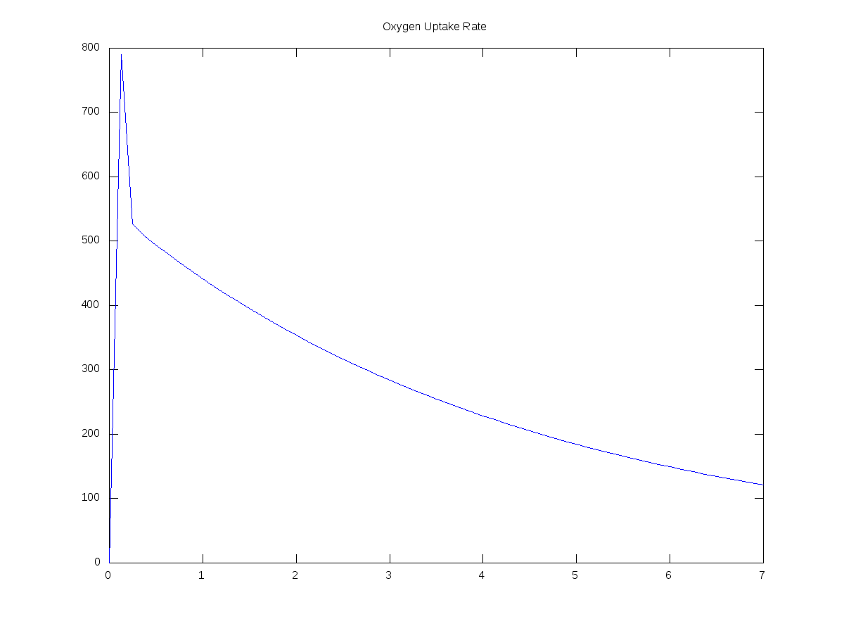
OUR = -1*Ct(:,8);
plot(Timet,tCOD,'r-');
title('Total COD');
figure;
plot(Timet,MLVSS,'g-');
title('Biomass');
figure;
plot(Timet,OUR,'b-');
title('Oxygen Uptake Rate');
%Type 'figure(1)', 'figure(2)', 'figure(3)' to cycle back through figures
%With a figure selected, save it using the command 'print('filename.png','-dpng')'
Input and Output
Here are some graphs produced from the script above, together with the input values I used:
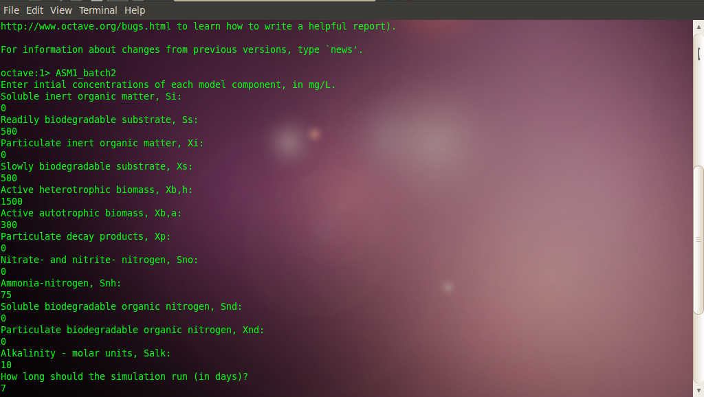
(Units are days and mg/L)
On a different topic...
In the simplified mark-up language that ghost (i.e. this blogging platform) uses, blocks of code should be preceded by 4 spaces. These can be added efficiently in a bash terminal using sed: cat ASM1_batch2.m | sed 's/^/ /'