Deffeyes Diagram

This post is intended to complement the previous one with a more theoretical look at dissolving carbon dioxide in water.

I wrote a script in R to draw a Deffeyes diagram. This diagram shows the interplay between CO2, pH, and alkalinity. My main reference was the venerable Water Chemistry textbook by Snoeyink and Jenkins (1980).

Here is the script:

#Deffeyes.R - an R script to produce the Deffeyes alkalinity-pH-carbonate diagram
#
# By Daniel B. Scott
#
# Description: the Deffeyes diagram shows carbonate concentration (in mmol/L) on the x-axis, the 
# total alkalinity (in meq/L) on the y-axis, and the pH as lines within the plot. If two of the 
# variables are known the third can be determined. Some common chemical additions to alter these
# parameters can be calculated as simple movements on the plot. 
#
# Variables: 
# pH.low, pH.high, pH.int: range and step size for pH values on plot
# Kacid1, Kacid2: Ka (acid dissociation) values for HCO3^- and CO3^2- respectively
# Kwater: equilibrium constant for H+ and OH-
# CO3.max, CO3.int: range and step size for carbonate concentrations on plot
# n.records: the length of the ``Records'' vectors
# Record$CO3, Record$pH, Record$TAlk: carbonate concentrations, pH values, and Total alkalinities to use on plot
# i: an index counter
# pH.curr, CO3.curr, TAlk.curr: pH values, carbonate concentrations, and total alkalinities calculated within loop
# alpha1, alpha2: distribution coefficients for HCO3^- and CO3^2- respectively
# denom: denominator in alpha1 and alpha2 calculations
# pH.line: loop index counter for plotting


##START OF CALCULATIONS
#Input constants and ranges and set-up variables
pH.low <- 5.5
pH.high <- 10.0
pH.int <- 0.2
Kacid1 <- 10^(-6.42) #using values for 15 C from Table 4.7 in Snoeyink and Jenkins (1980)
Kacid2 <- 10^(-10.43) #using values for 15 C from Table 4.7 in Snoeyink and Jenkins (1980)
Kwater <- 10^(-14)
CO3.max <- 4.0
CO3.int <- 0.5

n.records <- (((pH.high - pH.low)/pH.int) + 1)*((CO3.max/CO3.int)+1)
Record <- data.frame(CO3 = numeric(n.records), pH = numeric(n.records), TAlk = numeric(n.records))
i <- 1 # index for Record dataframe

#Loop through calculations
for (pH.curr in seq(pH.low,pH.high,pH.int)) {
  denom <- (10^(-1*pH.curr))^2 + (10^(-1*pH.curr))*Kacid1 + Kacid1*Kacid2
  alpha1 <- (10^(-1*pH.curr))*Kacid1/denom
  alpha2 <- Kacid1*Kacid2/denom
  for (CO3.curr in seq(0,CO3.max,CO3.int)) {
    TAlk.curr <- CO3.curr*(alpha1+2*alpha2) + 1000*(Kwater/(10^(-1*pH.curr)) - (10^(-1*pH.curr))) #factor of 1000 to convert [H+] and [OH-] to mmol/L
    #record calculations
    Record$CO3[i] <- CO3.curr
    Record$pH[i] <- pH.curr
    Record$TAlk[i] <- TAlk.curr
    i <- i + 1
  }
}

#Plot Deffeyes diagram 
png("Deffeyes.png", width=960,height=840)
par(mar=c(5,5,5,5),cex=0.85)
plot(Record$CO3, Record$TAlk, type="n", xlab="Carbonate concentration (mmol/L)", ylab="Total Alkalinity (meq/L)", xlim=c(0,CO3.max), ylim=c(0,CO3.max)) #set-up plot
#place pH lines (with labels)
for (pH.line in seq(pH.low,pH.high,pH.int)) {
  lines(Record$CO3[Record$pH==pH.line], Record$TAlk[Record$pH==pH.line], lty=1)
  text(median(Record$CO3[Record$pH==pH.line]),  median(Record$TAlk[Record$pH==pH.line]), labels=as.character(pH.line))
}

dev.off()

Here is the diagram:

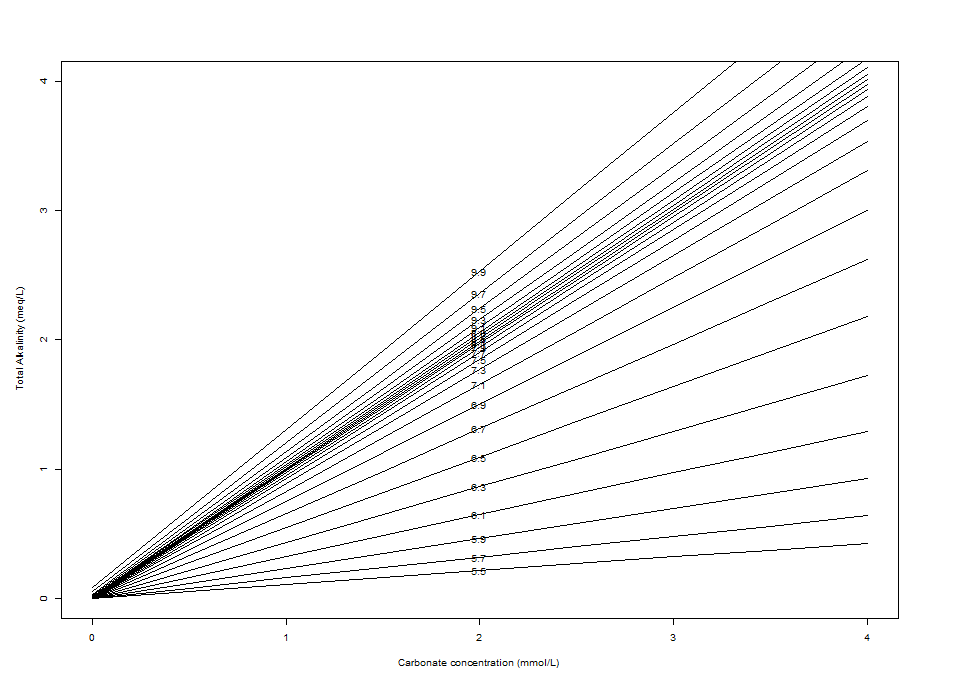
The total carbonate concentration is shown on the x-axis, the total alkalinity (in meq/L; 1 meq = 50 mg/L as CaCO3) is shown on the y-axis, and the lines indicate pH values. Note that the quantity on the x-axis includes not only dissolved CO2 (i.e. CO_2(aq)), but also bicarbonate and carbonate ions. The Henry's Law calculations in my post last week only give the dissolved CO2 concentration, but at neutral or higher pH values the amount that dissociates into ions will be significant—so my CO2 cylinder probably won't last as long as predicted.

Adding a strong acid or strong base means moving down or up (respectively) the y-axis, while adding CO2 (e.g. by increasing the concentration of CO2 in the gas phase over the water) at a constant alkalinity means moving along the x-axis; additions of chemicals that contribute both carbonate and alkalinity (e.g. sodium bicarbonate or calcium carbonate) require diagonal movements. Diluting the solution requires a 1:1 movement toward the origin. Since the pH lines have different slopes, dilutions can change the pH of the solution. Determining the post-dilution pH can be a lot easier graphically using the Deffeyes diagram than by doing calculations.

I also made another version of the diagram at higher ranges of carbonate and alkalinity concentrations to try to be relevant to anaerobic wastewater treatment:

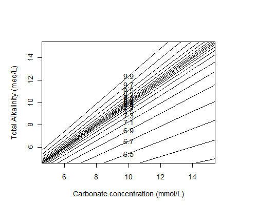
It should actually have a higher range than it does: 12 mmol/L of carbonate is only the amount of dissolved CO2 (so not counting bicarbonate and carbonate ions, which will be significant at the pH values shown) given by Henry's Law, at a CO2 partial pressure of 0.35 atm which is typical for the headspace of an anaerobic digester.

It would be interesting to add calculations to the script above to calculate the corresponding gas phase CO2 partial pressure from the total carbonate and the pH (using Henry's Law and dissociation constants) and use that on the x-axis instead.

Aside from the carbonate system, phosphate, sulfate, and volatile organic acids are also involved in alkalinity/buffering pH. I don't know how valid this diagram is in situations where their concentrations are significant.

Permalink