Hilbert Curve

One of my favourite topics in math is fractals. For this post, I drew the Hilbert Curve fractal in octave.

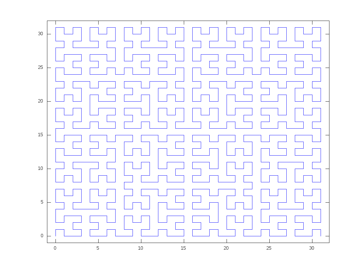
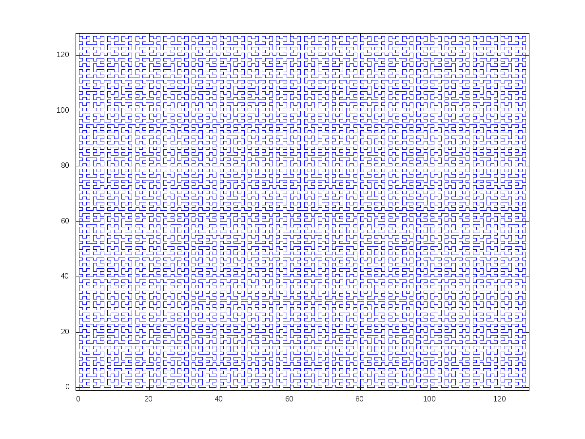
The Hilbert Curve is a space-filling curve: although it is one-dimensional (a series of line segments) itself, it covers a two-dimensional area. I recently learned about this fractal from a post on Andrea Hawksley's blog.

(Her blog also has some other math art and some ideas for playing chess and Carcassonne on non-Euclidean boards (i.e. not on flat grids)).

To draw the Hilbert Curve, I wrote a script in octave to implement the Lindenmayer system algorithm from Wikipedia. The results are shown below, after 5 and 7 iterations, respectively. The script I wrote is included at the end of this post.

With its space-filling properties, the Hilbert Curve has some commonalities with tiling, another mathematical topic that really interests me. I really like the aesthetics of this fractal.

Images

Octave Code

%% Hilbert.m - this is a script to draw the space-filling Hilbert curve. 
% From Wikipedia, the algorithm is as follows: 
% A = - B F + A F A + F B -
% B = + A F - B F B - F A +
% Where: F indicates move forward, - is a left turn (which actually should 
%  be positive, using the right hand rule), + is a right turn, and A and B
%  are place-holders that are expanded as indicated above on each iteration.
% (In the script below, numbers 1 - 5 are used for A, B, -, +, and F, 
%  respectively)
% This script has 3 parts: 1. generate the instruction list to the depth 
%  (number of iterations) desired. 2. calculate the coordinates of each 
%  vertex on the curve. 3. plot the curve. 


%% Generate the instruction list

A = [ 3 2 5 4 1 5 1 4 5 2 3 ];
B = [ 4 1 5 3 2 5 2 3 5 1 4 ];
Depth = input("How many iterations? \n");
InstList = A;
Iter = 1; 

while Iter < Depth 
	InstListNew = []; %start with a blank list to fill in
	for Item = 1:length(InstList)
		switch (InstList(Item)) 
			case 1
				InstListNew = [ InstListNew, A ]; %expand the instruction list where appropriate
			case 2 
				InstListNew = [ InstListNew, B ];
			otherwise
				InstListNew = [ InstListNew, InstList(Item) ];
		endswitch
	end
	InstList = InstListNew;
	Iter = Iter + 1;
end


%% Calculate the vertex coordinates

R3 = [ 0 -1; 1 0 ]; %rotation matrix for left turn ("3" in instruction list)
R4 = [ 0 1; -1 0 ]; %rotation matrix for right turn ("4" in instruction list)
dir = [ 1; 0 ]; %initial direction vector points along the x-axis
posx = 0; %initial position is (0,0)
posy = 0;  

xpts = [ posx ]; %initialize x and y vectors, plus distance tally and a step counter
ypts = [ posy ];
distance = [ 0 ];
step = 1;

for Index = 1:length(InstList)
	switch (InstList(Index))
		case 3
			dir = R3*dir; %rotate left
		case 4 
			dir = R4*dir; %rotate right
		case 5 
			posx = posx + dir(1); %move forward in the direction currently faced. 
			posy = posy + dir(2); 
			step = step + 1; 
			xpts(step) = posx; %record current position
			ypts(step) = posy; 
			distance(step) = (step - 1); %record cumulative distance travelled
	endswitch
end

%% Draw the curve
plot(xpts,ypts,'b-'); %plot the recorded points 
xlim([-1, (max(xpts)+1)]);
ylim([-1, (max(ypts)+1)]);

%It might also be of interest to plot x and/or y vs the distance travelled 
% (commented out for now)
%plot(distance,xpts,'g-');
%plot(distance,ypts,'r-');

%Note: save the figure using the command 'print('filename.png','-dpng')' 

Permalink