Ticket to Ride's Adjacency Matrix
As promised, here is a post analyzing strategy for a board game: Ticket To Ride—one of my favourites.
Analysis
I had fun learning a bit more about graph theory and using it for the calculations in this section, but if you're just interested in the results as they apply to Ticket to Ride strategy, feel free to skip to the second section.
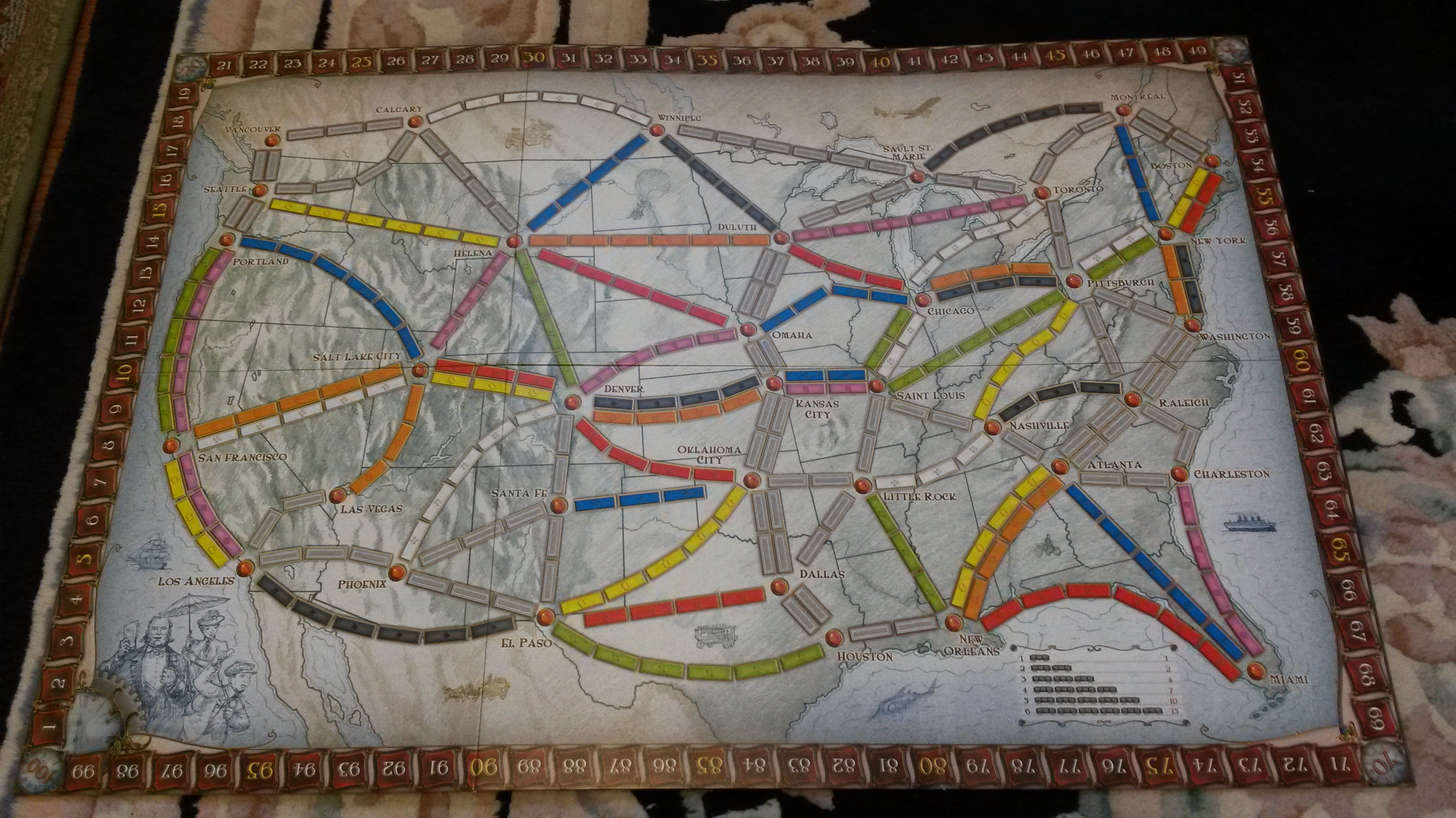
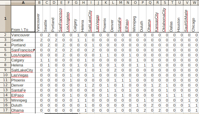
To analyze the Ticket to Ride board (shown below) for some strategic locations and routes, I started by representing it mathetically with an adjacency matrix. An adjacency matrix lists the number of edges (train routes on the board game) connecting every pair of vertices (hub cities on the board game) at the intersection of the corresponding row and column. In my matrix, a portion of which is shown in the second image below, vertices/cities are ordered from north to south and west to east. So cell (1,2) lists the two routes (I've counted both parallel tracks, which are "in-play" with 4 or 5 players) connecting Vancouver and Seattle. Since the map is an undirected graph, its adjacency matrix is symmetrical and cell (2,1) also equals 2.
I imported the full adjacency matrix into octave and did some calculations on it that I thought would be interesting. The glossary of graph theory from Wikipedia was a useful reference.
The degree of a vertex (city) is the number of edges (routes) connected to it; it quantifies how well-connected the points on the map are. The total degree is the sum of the degrees of each vertex and equals two times the number of edges. The Ticket to Ride board is an irregular graph since not every vertex has the same degree.
Here are some calculations related to the degree of vertices and the overall graph:
octave:7> sum(TTRAdj)
ans =

 Columns 1 through 31:

   3   6   5   6   5   4   7   7   2   4   9   4   6   4   7   7   8   8   6   4   4   7   7   5   5   5   5   9   7   5   4

 Columns 32 through 36:

   7   5   7   3   3

octave:8> sum(sum(TTRAdj))
ans =  200
octave:10> for r=1:36
> rowsum(r)=sum(TTRAdj(r,:));
> end
octave:11> max(rowsum)
ans =  9
octave:14> for r=1:36
> if rowsum(r)==9
> fprintf("%f \n",r);
> end
> end
11.000000
28.000000
octave:15> %11 is Denver and 28 is Pittsburgh
octave:29> sum(TTRAdj) < 5
ans =

 Columns 1 through 31:

   1   0   0   0   0   1   0   0   1   1   0   1   0   1   0   0   0   0   0   1   1   0   0   0   0   0   0   0   0   0   1

 Columns 32 through 36:

   0   0   0   1   1

octave:30> sum(ans)
ans =  11
octave:31> %Only 11 cities/hubs have a degree less than 5--blocking opponents is difficult
Looking at the degree of each point, it can be seen that it ranges from 3 – 9; the total degree is 200. The cities with the highest degree are Denver and Pittsburgh. Only 11 cities have a degree less than 5 (the maximum number of players), so there is room for each player to have at least one connection to most cities— blocking someone from completing a route is difficult (but not impossible, as Ticket to Ride players will know).
The radius and diameter of a graph are defined as follows. The radius the minimum number of edges (train route legs in the game) to connect a vertex (city)—the most central one—to all others. The diameter is the minimum number of edges that will connect the two vertices that are furthest apart. As mentioned above, the adjacency matrix lists the number of connections between pairs of vertices. It also has the useful property that when it is multiplied by itself N times, the product shows the number of connections comprising N segments (train route legs). I did this in octave, as shown below, to find the radius and diameter:
octave:15> MultiLeg = TTRAdj * TTRAdj;
octave:16> legs = 2;
octave:21> while max(min(MultiLeg)) < 1
> MultiLeg = MultiLeg * TTRAdj;
> legs = legs + 1;
> end
octave:22> legs
legs =  4
octave:23> min(MultiLeg)
ans =

 Columns 1 through 31:

   0   0   0   0   0   0   0   0   0   0   0   0   0   0   0   0   6   0   0   0   0   1   0   0   0   0   0   0   0   0   0

 Columns 32 through 36:

   0   0   0   0   0

octave:24> %17 is Kansas City, which can reach the most distant point in 4 legs
octave:24> MultiLeg(17,:)
ans =

 Columns 1 through 20:

    12    26    36    40    42    26   150   146    16    80   198   130    98    36   156   138   428   136   148    36

 Columns 21 through 36:

    34   212    80   126    22    80    42   104    22    20     8    32    30    28     6     6

octave:25> %there are 6 4-leg journeys from KC to Miami and Charleston
octave:25> %22 is Chicago, which can also reach the most distant point in 4 legs
octave:25> MultiLeg(22,:)
ans =

 Columns 1 through 20:

     7    10     8     8     1    16    87    39     4    17    84    32    19    41   124   107   212    47    36     6

 Columns 21 through 36:

    59   247   114    71    22   111   101   156    37    59    40   145    87   100    19    12

octave:26> %The most distant point from Chicago is Los Angeles (only 1 possible route of 4 legs)
octave:26> while min(min(MultiLeg)) < 1
> MultiLeg = MultiLeg * TTRAdj;
> legs = legs + 1;
> end
octave:27> legs
legs =  7
octave:28> %The diameter of the Ticket to Ride North America "graph" (map) is seven--the most distant points can be joined with that many edges
octave:28> min(MultiLeg)
ans =

 Columns 1 through 17:

      3     81     65    138    102     90    706    543     69    502   2034    802    616    312   1652   2245   3330

 Columns 18 through 34:

   3004   1097    418    712   2452   2655    819    129    506   1157   1519    104    317    102    377    291    247

 Columns 35 and 36:

     19      3

octave:29> %Vancouver and Miami are the furthest apart points (only 3 possible routes connecting them with 7 hops)
The radius of this graph is 4. Chicago (with Los Angeles as the most distant point) and Kansas City (with Miami and Charleston as the most distant points) are the central cities—any other city can be reached with no more than four connections from either of these cities. The diameter of the graph is 7, which is how many edges (train route legs) that it takes to connect Miami to Vancouver.
Eigenvalues of an adjacency matrix are significant in spectral graph theory. I only did a little bit of reading on this topic for this post, but I learned a couple of things:
- For a symmetrical matrix, all of the eigenvalues will be real, and
- The largest eigenvalue will be the average degree or maximum degree or somewhere in between (from section 16.6 here).
In some calculations in octave I found both of these statements to be the case (the largest eigenvalue was 6.45 and the average degree was 5.56; 5.56 ≤ 6.45 ≤ 9.00):
octave:5> eig(TTRAdj)
octave:6> max(eig(TTRAdj))
ans =  6.4503
octave:31> 200/36
ans =  5.5556
Something I didn't calculate is the Cheeger constant which is related to bottlenecks in the graph. A visual examination of the board doesn't show any obvious bottlenecks, but if there were some, they'd be strategically important. Regular graphs (recall that this one is irregular) have a convenient inequality involving one of the eigenvalues that can narrow down the value of the Cheeger constant. Further eigenvalue-based analysis could be performed if I calculated the Laplacian matrix (which is the negative of the Adjacency matrix with the degree of each vertex added along the diagonal).
Application
The analyses above suggest some strategy ideas for Ticket to Ride, although I haven't had a chance to play-test them yet:
- Chicago and Kansas City might be good starting points for a hub-and-spoke strategy, since from these locations any other city can be reached with 4 or fewer route segments. This is a case of art imitating life, as the US Midwest is the centre of a lot of rail activity.
- It takes more route segments to join up Miami and Vancouver than any other pair of cities, so players aiming for the longest route achievement might want to include them in their strategy.
- The cities of Miami, Charleston, Los Angeles, and Vancouver are more distant from the central cities, so connecting them is worth more points, with good reason!
- With their high degree, Denver and Pittsburgh might be safe to leave unconnected until late in the game since it will be hard for other players to shut you out of those cities.
Finally, it should be noted that I didn't consider the length of routes in my analyses. Depending on the cards you get, you might need to utilize more shorter routes rather than the most direct connections.