Water Quality Profile Along an Entire River

I previously blogged about an expedition to travel the entire length of the Rio Grande, by reporter Colin McDonald. That expedition has now come to an end, having reached its destination: the Gulf of Mexico.

Introduction

The Disappearing Rio Grande Expedition (DRGE) collected a lot of water quality data along the way. Since they made this data publicly available on the expedition's blog, I thought it would be a great opportunity to analyze how several water quality parameters varied along the length of an entire river.

First, a few important caveats:

• These parameters were measured with field kits/instruments, not in a certified lab.
• Samples are from a single point in space and time (i.e. grab samples); they don't necessarily represent the average water quality at each location along the Rio Grande.
• At least one or two of the samples were collected from tributaries rather than the Rio Grande itself. Also, at least one sample required digging a pit because the river channel had no water in it.
• Finally, I'm not affiliated with the expedition in any way, beyond backing it on Kickstarter—I simply collected and analyzed the data published on their blog.

Method

To start with, I went through the expedition archives and entered the water quality measurements into a spreadsheet, with a row for each day of the expedition on which samples were collected. There were a total of 71 measurements, over an elapsed time of 219 days. In the graphs below, the x-axis is in days. The expedition had some days off (e.g. over Christmas) and some side trips (for interviews, etc.), so the analysis could be extended by replacing the elapsed time with the distance travelled as the independent variable, but that would require a lot more work to calculate. In the spreadsheet, I cleaned up some data points that appeared to have the decimal point in the wrong place, and also recorded "N/A" for times when certain instruments weren't working properly—anyone who's ever used a portable pH meter can appreciate how finicky they are sometimes!

I used the Benson and Krause equations (see page 6 of this USGS memo) to calculate the solubility of oxygen in water for the conditions from each day, with the following assumptions:

• Salinity (as TDS in mg/L) calculated by multiplying conductivity measurements by a rough empirical factor of 0.61 (0.64 might have been better to use).
• To estimate atmospheric pressure, I assumed that the elevation varied linearly from 13,500 ft ASL to 7,500 ft ASL upstream of Alamosa, Colorado (Day 15) and linearly from 7,500 ft ASL to 0 ft downstream; I used Alamosa as an inflection point since Colin McDonald mentioned the elevation there. From the elevation, I calculated pressure with the following equation:

The difference between oxygen solubility and the actual measured dissolved oxygen concentration (known as an oxygen deficit) indicates where oxygen is being used up—normally via the degradation of organic matter—more quickly than it can re-dissolve from the atmosphere. See here and here for more background. Use this online widget to calculate oxygen solubility under different conditions.

Then I imported the spreadsheet into R for analysis. In R, I calculated some non-parametric correlations and prepared some plots.

Graphs

Air (*) and Water Temperature (~)

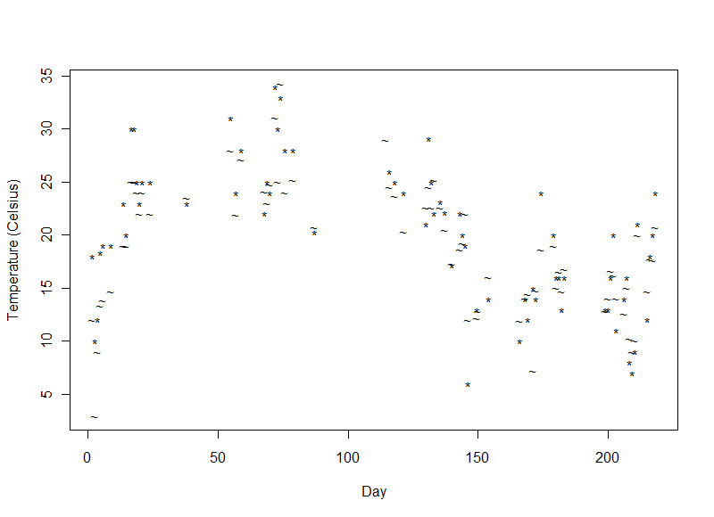
The air and water temperatures were similar to each other. They varied with the time of year (since the expedition began in June 2014 and ended in January 2015) and were also lower at the start of the expedition high in the Rockies.

Conductivity (+)

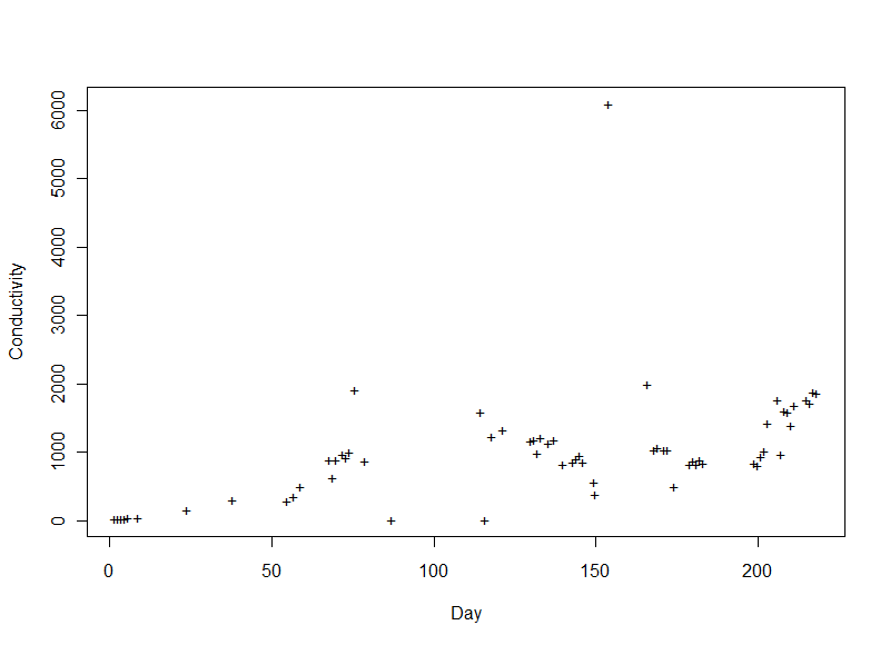
Conductivity is influenced by the amount of dissolved matter in the water. It increases as the river picks up more salts/minerals and organic matter along its journey. Where it meets the Gulf, the tide could bring some salt upstream from the sea a bit. One day had a conductivity far higher than the rest (around 6,000 μS/cm); on that day the expedition had observed some fish kills from an algal toxin. The increased conductivity may have been from dissolved material secreted by the algae and/or released from decaying fish.

Base-10 logarithm of E. coli colony counts (X)

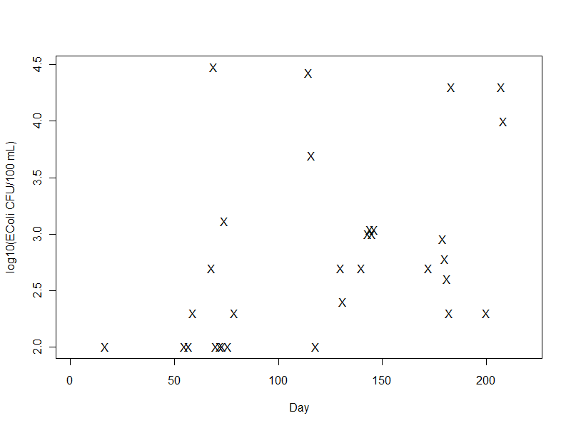
E. coli colonies detected with a test kit varied over several orders of magnitude, so they're plotted on a logarithmic axis. Samples that were below the detection level are not plotted.

Dissolved Oxygen Depletion (O)

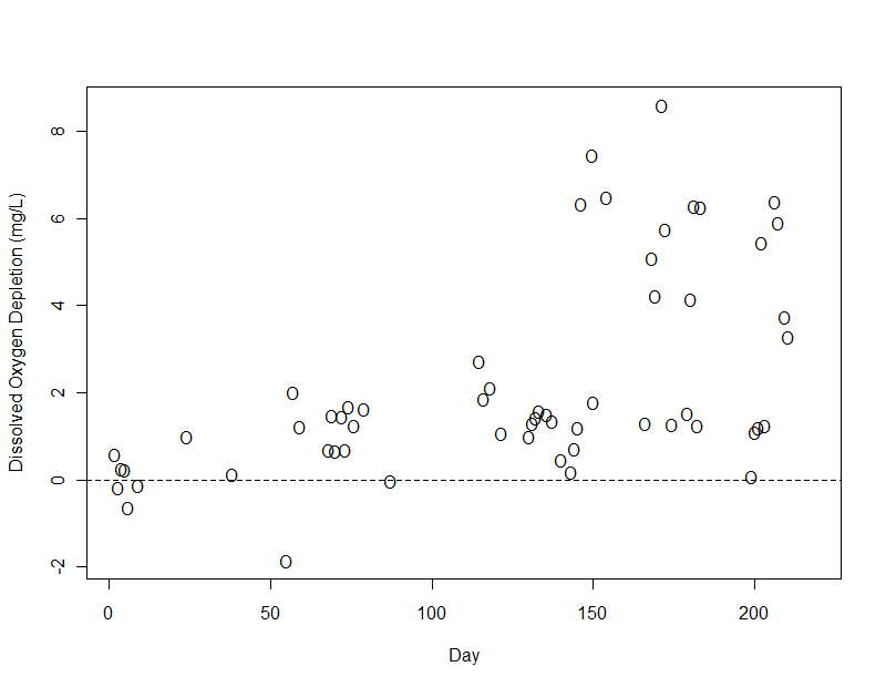
The dissolved oxygen (DO) deficit was low (median < 2 mg/L) in most samples. A higher deficit was observed on some days in the lower reaches of the river. In this plot, a dashed line indicates zero depletion (i.e. measured DO equal to its solubility). The clustering around this line, especially in the pristine, well-oxygenated mountain waters, suggests that the solubility calculations were reasonably accurate.

To put these graphs in context, here are some days of the expedition that correspond to significant places:

• Day 2 = Stoney Pass, CO
• Day 15 = Alamosa, CO
• Day 30 = Colorado – New Mexico border
• Day 59 = Albuquerque, NM
• Day 76 = Hatch, NM
• Day 87 = El Paso, TX
• Day 169 = Amistad Dam
• Day 202 = Rio Grande City, TX
• Day 215 = Brownsville, TX

I'll just remark here that it would have been nice to have some nutrient data (e.g. ammonia, nitrate, and phosphate) to consider the issue of eutrophication—especially vis-à-vis the algal bloom that was observed.

Statistics & Correlations

This section gets pretty detailed, so skip ahead if you're not interested in statistics.

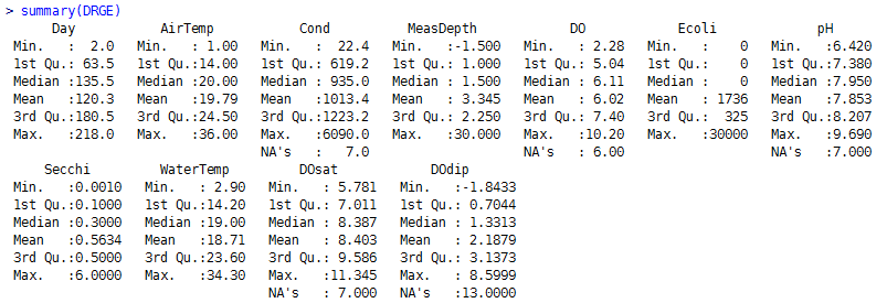
First, here are some basic summary statistics for each parameter included in my analysis.

I then calculated non-parametric Spearman correlations between parameters:

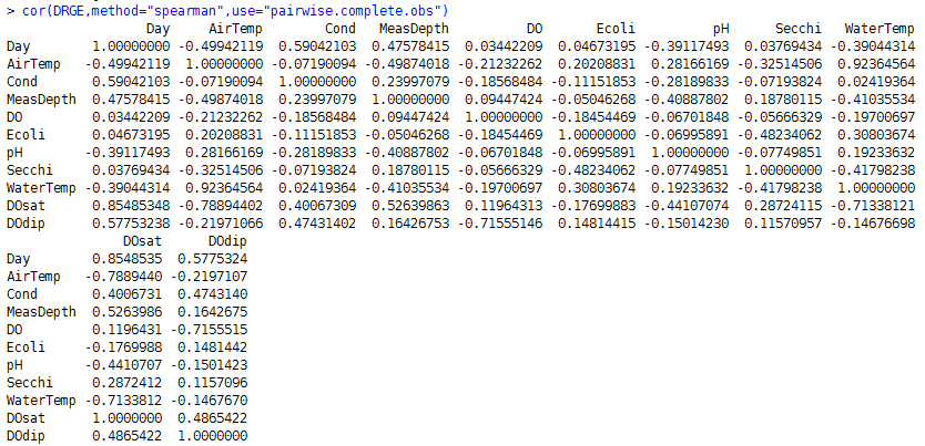
A positive correlation between a pair of parameters indicates that they generally increase together while a negative correlation indicates that one generally decreases when the other increases (and vice versa). A greater magnitude indicates a stronger correlation. Unlike the more commonly-used Pearson correlation (familiar from the R² statistic), Spearman correlations don't assume a linear relationship.

The previous table doesn't indicate which correlations are statistically significant, so I looked at some of them in more detail.

> cor.test(DRGE$DOdip,DRGE$Cond,method="spearman")

	Spearman's rank correlation rho

data:  DRGE$DOdip and DRGE$Cond 
S = 17089.53, p-value = 0.000169
alternative hypothesis: true rho is not equal to 0 
sample estimates:
     rho 
0.474314 

Warning message:
In cor.test.default(DRGE$DOdip, DRGE$Cond, method = "spearman") :
  Cannot compute exact p-values with ties
> cor.test(DRGE$AirTemp,DRGE$WaterTemp,method="spearman")

	Spearman's rank correlation rho

data:  DRGE$AirTemp and DRGE$WaterTemp 
S = 4553.774, p-value < 2.2e-16
alternative hypothesis: true rho is not equal to 0 
sample estimates:
      rho 
0.9236456 

Warning message:
In cor.test.default(DRGE$AirTemp, DRGE$WaterTemp, method = "spearman") :
  Cannot compute exact p-values with ties
> cor.test(DRGE$Cond,DRGE$Day,method="spearman")

	Spearman's rank correlation rho

data:  DRGE$Cond and DRGE$Day 
S = 17890.41, p-value = 2.82e-07
alternative hypothesis: true rho is not equal to 0 
sample estimates:
     rho 
0.590421 

Warning message:
In cor.test.default(DRGE$Cond, DRGE$Day, method = "spearman") :
  Cannot compute exact p-values with ties

The above correlations were all significant at the 0.05 level. They all make sense according to what would be expected, too. Conductivity and the oxygen deficit generally increase together, as do air and water temperatures, and conductivity with the day of the expedition. As more dissolved material flows into the river (e.g. run-off from fields), the conductivity will increase, and as the organic portion of this material is degraded, oxygen will be consumed. The water temperature is strongly influenced by the air temperature, of course. And the conductivity generally increases going downstream (seen in the second figure) since material dissolved upstream can keep accumulating along the course of the river.

One final example shows the usefulness of applying a non-parametric analysis:

> cor.test(DRGE$Ecoli,DRGE$Secchi,method="spearman")

	Spearman's rank correlation rho

data:  DRGE$Ecoli and DRGE$Secchi 
S = 88406.8, p-value = 2.049e-05
alternative hypothesis: true rho is not equal to 0 
sample estimates:
       rho 
-0.4823406 

Warning message:
In cor.test.default(DRGE$Ecoli, DRGE$Secchi, method = "spearman") :
  Cannot compute exact p-values with ties
> cor.test(DRGE$Ecoli,DRGE$Secchi,method="pearson")

	Pearson's product-moment correlation

data:  DRGE$Ecoli and DRGE$Secchi 
t = -1.3, df = 69, p-value = 0.1979
alternative hypothesis: true correlation is not equal to 0 
95 percent confidence interval:
 -0.37441483  0.08163111 
sample estimates:
       cor 
-0.1546173 

The Spearman correlation (non-parametric) between the Secchi disk visibility depth and E. coli count was found to be significant at the 0.05 level while the Pearson correlation (parametric) was not. As is typical for microorganisms, the E. coli data is not normally distributed, but rather exponentially explodes in a relatively small number of samples. Its non-linear behaviour makes it poorly suited for statistics that assume otherwise. The Secchi disk visibility depth decreases when the turbidity (caused by particles suspended in the water) increases. It makes sense that the E. coli counts would often increase under the same conditions (giving the negative correlation observed). For example, agricultural run-off could add both sediment particles and E. coli to the river water.

Next Week

On a semi-related note, I'm excited to have the opportunity to attend a conference on water reuse in Austin, Texas early next week (February 1 – 3). Watch for an upcoming post about my experiences there.

Permalink