Nomography
Nomography is the art/science (both are involved) of graphical calculators. Using a nomogram, you can quickly solve an equation (but only the one it was designed for) with the aid of nothing more than a straightedge. It's something I've been interested in for quite a while, and finally feel that I have the material to make a good (hopefully!) post about it.
Introduction
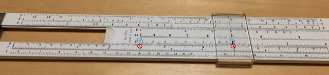
I'll begin this post by talking about slide rules, because more people are probably familiar with them, and they share some mathematical principles with nomography. Slide rules have a number of different scales that can slide against each other. By aligning them in certain ways, you can perform various calculations. It's perhaps easy to see how they could be used for addition or subtraction: since those operations can be thought of as moving up or down a number line, offsetting two linear scales the correct distance from each other will deliver the result. For multiplication (and division), slide rules use the trick that logarithms turn multiplications into additions: the log of a product is the sum of the logs of its factors. (Logarithms also turn exponents into products). In the image below, a slide rule is being used to multiply 2.5 × 2; the operation can also be thought of as similar ratios (1:2.5 :: 2:5).
Nomography was only popular for slightly more than half a century. It was largely developed in the final decades of the 1800s, and waned after the invention of electronic calculators in the 1960s. As I said, it uses similar principles as slide rules. A big difference is that slide rules were general purpose (the scales could be slid against each other) while nomograms, being stationary graphics, were configured to solve a single equation.
There are various types of nomograms, but I'm only going to focus on the two that I think are the most useful: alignment nomograms with parallel axes, and "N" (sometimes called "Z") nomograms. The former are used to solve linear equations (or equations that can be linearized, as already noted) of three variables (and they can be compounded together to handle more variables) and the latter are used when one variable is the quotient of the other two (or the quotient of functions of the other two).
Visualize three parallel lines (equally spaced), A, B, and C. If a straight line is drawn that intersects all three, the height at which it crosses B (the middle line) will be the average of where it crosses A and C. Stated as an equation, B = (A + C)/2 or A + C - 2B = 0. A basic nomogram can be created simply by rearranging an equation of interest into the same form, pairing its variables up with A, B, and C, and marking out the applicable scales on each line (not neglecting the factor of -2 that alters the scale on B). For example, the equation X × Y = Z can be linearized by taking the logarithm of each side and rearranged to log X + log Y - log Z = 0. Matching it with the earlier equation (this process reminds me of "destructuring" in Clojure) gives A = log X, C = log Y, and -2B = -log Z (or B = 0.5 log Z)—the nomogram is completed by marking each line with the scale stated by these paired-off equations.
Another way of looking at nomograms is through the geometry of similar triangles. This is explained here (the first post in a series that was a major source of information for my own post). This technique can be used in the construction or analysis of parallel or N type nomograms.
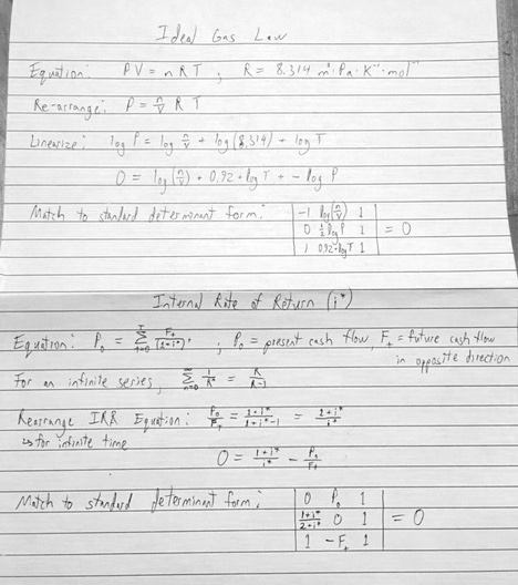
A more powerful and general technique involves the use of determinants. The equation of interest is put into a standard determinant form:
| X(a) | Y(a) | 1 |
| X(b) | Y(b) | 1 |
| X(c) | Y(c) | 1 |
As mentioned in the linked post (which is from another series that was a major resource for this post), the value of the determinant is zero, each row has equations of only one variable (this can require more "destructuring"), and the final column is all 1s. There are a number of valid manipulations ("four rules") that can be done to adjust determinants into this form. Once it is in the required form, the first two columns of each row are parametric equations that relate the x and y coordinates of each line or curve in the nomograph to a variable (one variable per line/curve) in the original equation (these variables are represented by a, b, and c in the table above).
The book by Dr. H.A. Evesham referenced below says:
Given a relationship F(x,y,z) = 0, can it be expressed in the determinant form given?
If it can, then an alignment nomogram can be constructed. (p.79)
The standard determinant form acts as a sort of bridge between the equations derived from the geometry of the lines of the nomogram (see the discussion above) and the equation you're trying to make a nomogram for, since they can both be mapped to this determinant structure (if making a nomogram is possible).
The main part of this post will give some instructions and examples for the determinant method of constructing nomograms.
Instructions
- Do some algebra to tidy up your equation. This will commonly involve moving all of the variables and constants to one side (so it is equal to zero), replacing named constants with their numerical value, and linearizing (i.e. taking the logarithm to convert multiplications to additions). If there are more than three variables, split it into multiple equations (by introducing new place-holder variables). The resulting nomograms can later be compounded together.
- Rather than re-invent the wheel, check to see if the structure of your equation fits one of the forms on this page*. If it does, use the determinant given. Otherwise, you have to figure out how to get it into a determinant in the standard nomographic form on your own.
- Manipulate the determinant as needed. This may involve adding functional moduli (outside the scope of this post) and/or transforming it in some way (in one of my examples below, I multiply by a shear matrix). This will probably be an iterative process; return to this step to improve the appearance of a nomogram by trying different manipulations on the determinant.
- For each variable, select the range that will be covered by the nomogram.
- Plot the lines/curves of the nomogram using the parametric equations X(a), Y(a); X(b), Y(b); and X(c), Y(c). In my examples below, I did steps 4 and 5 in R.
Like I said, it can be an iterative process to get something that looks good and has useful resolution in the key parts of the range.
*Here are the basic nomographic forms for parallel and N type nomograms from the "cheat sheet" linked to earlier:
Parallel type: For an equation of the form f(a)+f(b)+f(c)=0, the determinant (also equal to zero) is:
| -1 | f(a) | 1 |
| 0 | -0.5 f(b) | 1 |
| 1 | f(c) | 1 |
N type: For an equation of the form f(a)-f(b)/f(c)=0, the determinant (also equal to zero) is:
| 0 | f(b) | 1 |
| f(a)/{f(a)+1} | 0 | 1 |
| 1 | -f(c) | 1 |
(this actually gives perpendicular lines rather than a proper N, unless a shear factor is applied)
In order to verify that the determinants are correct, they can be expanded to check that the original equation is returned. I like the method described here of adding up the products of the diagonals from top-left to bottom-right and subtracting the products of the diagonals from top-right to bottom-left, wrapping around in both cases.
Examples
The following examples are of the Manning formula, Froude number (these first two were featured in a post I wrote earlier this year), the Ideal Gas Law, and the internal rate of return (IRR) of a perpetuity. Note that the first three are all in standard SI units.
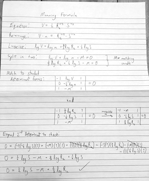
For this one I made two nomograms with a match line and pasted them together in an image editor (which made the pasted side blurry, unfortunately). The lines crossing the two scales on either side of the match line should intersect on the match line. This is an example of how alignment nomograms can be compounded together to use more than three variables. Also note that it uses the simplification that the hydraulic radius is approximately equal to the depth when the width is much greater than the depth.
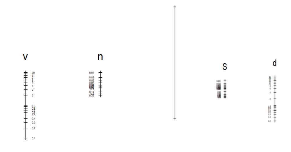
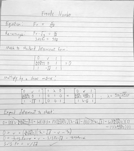
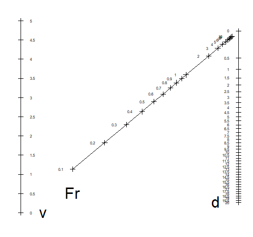
The Froude number determinant was multiplied by a shear matrix so that the proper N shape would result. The spacing on the scale for the depth (d) is irregular because the equation uses the square root of the variable.
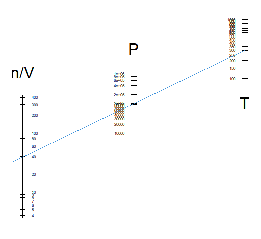
To reduce the ideal gas law to three variables, I treated n/V (i.e. the concentration, or the inverse of the molar volume) as a single variable.
The ideal gas law nomogram has a line added (at SATP conditions) to show how a nomogram is used for calculations. Only two variables need to be known to draw a line like this, and the third/unknown variable can be read from the intersection point with the other scale.
Here is the R code I used to draw this nomogram (the other ones were similar aside from the variable ranges, the precise parametric equations used, and the labelling):
#Making nomograms with determinant method
# | X(a) Y(a) 1 |
# | X(b) Y(b) 1 | = 0
# | X(c) Y(c) 1 |
# X(i) and Y(i) are parametric equations for the nomogram axes

#Set variables and ranges
a_pts <- c(seq(4,10,1),seq(20,100,20),seq(200,400,100))
a_name <- "n/V"
b_pts <- c(seq(10000,100000,10000),seq(200000,1000000,200000))
b_name <- "P"
c_pts <- seq(100,1000,50)
c_name <- "T"

#Calculate axes from parametric equations in determinant
Xa <- rep(-1,length(a_pts))
Ya <- log10(a_pts)
Xb <- rep(0,length(b_pts))
Yb <- 0.5*log10(b_pts)
Xc <- rep(1,length(c_pts))
Yc <- 0.92+log10(c_pts)

#Plot the nomogram
plot(c(Xa,Xb,Xc),c(Ya,Yb,Yc),type="p",pch=3,axes=F)
lines(Xa,Ya)
lines(Xb,Yb)
lines(Xc,Yc)
text(Xa,Ya,labels=a_pts,pos=4,offset=1,cex=0.5)
text(Xb,Yb,labels=b_pts,pos=2,offset=1,cex=0.5)
text(Xc,Yc,labels=c_pts,pos=2,offset=1,cex=0.5)
text(max(Xa),max(Ya),labels=a_name,pos=3,offset=2,cex=2)
text(max(Xb),max(Yb),labels=b_name,pos=3,offset=2,cex=2)
text(min(Xc),min(Yc),labels=c_name,pos=1,offset=2,cex=2)
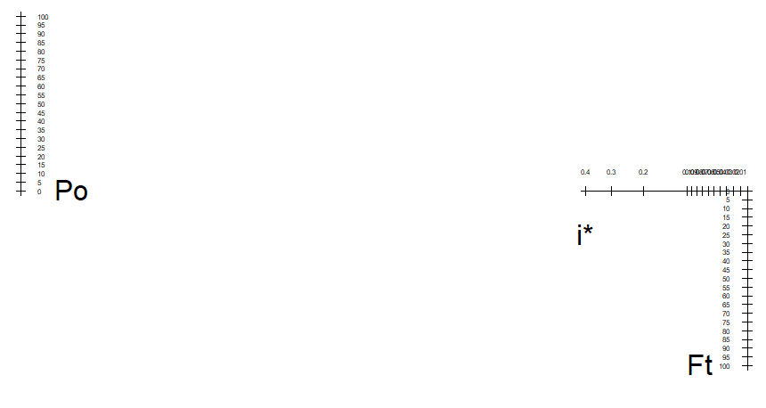
There was a mistake in the determinant for the internal rate of return (IRR) equation on the sheet of hand calculations that I discovered and corrected while plotting. Where it says {1+i}/{2+i} it should have been {1+i}/{1+2i} instead. This figure shows how an N-type nomogram is plotted if the basic determinant form is used without making any adjustments. If using this nomogram, note that it applies for cashflows that extend indefinitely into the future (e.g. spending Po on some home energy efficiency project now to save Ft monthly on your power bill). Also note that the way the equation is set up, the first instance of Ft occurs simultaneously with Po, so you'll need to subtract it from Po if comparing with other implementations of the IRR equation.
These nomograms could be improved by choosing the scale spacing more carefully to make the labels more legible and perhaps by playing with functional moduli or other manipulations to obtain more detail in key parts of the range.
Resources
- This site was an excellent walkthrough tutorial for learning the techniques I used here.
- The author has nomograms for the delta V rocket equation (briefly mentioned here) elsewhere on his site.
- The three blog posts starting here by Rod Doerfler were great for learning more of the theoretical background of nomography. The transformation examples in part III were very impressive.
- That author and some of his associates also have another site with some nomograms available.
- I also read part of the book The History and Development of Nomography by Dr. H.A. Evesham. It was adapted from his Ph.D. thesis, so the math was very dense in places, and I skipped or skimmed through more than half of it. But I did learn some of the history of the field from it. For example, Hilbert's thirteenth problem relates to nomography.
- A lot of the scholars who developed the field of nomography were from France. A name that comes up perhaps more than any other is Maurice d'Ocagne. Here is an excerpt from one of his books:
Si, aux diverses variables entrant dans une équation, on a fait correspondre respectivement des systèmes d'éléments géométriques, cotés au moyen des valuers de ces variables, et tels qu'entre les éléments correspondant à un ensemble de ces valeurs satisfaisant simultanément à l'équation donnée il existe une liaison graphique simple, d'une immédiate constatation à vue, on a réalisé une représentation graphique de cette équation qui permet, si l'on se donne les valeurs de toutes les variables moins une, d'avoir, par simple lecture, la valeur correspondante de cette dernière.
This paragraph basically explains about making a graphic representation of an equation and using it to read off an unknown variable when the values of the others are all known. One can certainly imagine the value of this kind of technique in a time before electronic calculators and computers were available.